
Application of Logistic Regression using R Programming
October 23, 2019
Multilevel Model Comparison and Statistical Diagnostics for Reliable Meta-Analysis Research
November 2, 2019APPLICATION OF TIME SERIES ANALYSIS IN FINANCIAL ECONOMICS
Summary:
Statistical techniques like Time Series Analysis allow the examination of an entity’s past behavior through historical data with the purpose of identifying trends, patterns and predicting future financial market opportunities. By using Time Series Analysis, the findings produced by any analysis conducted using Time Series Analysis can be utilized by investors, organizations and financial institutions as warranted in making sound investment decisions and create ways of forecasting future stock prices, interest rates, foreign exchange rates, among many other important global business/process indicators.
Markets are always changing; stock prices are always fluctuating, currencies may be affected by current global events, and interest rates will change according to the state of the economy [1]. To gain a better understanding of how markets perform, and to predict their future performance, experts require reliable methods for interpreting all of the data that communicates information about market performance, and time series analysis is one such tool used for this purpose.
With time series analysis, an analyst can examine historical data to find trends and patterns that can be used to predict potential future occurrences. Analysts can also use time series analysis to attempt to estimate where stocks may be heading, while using it to identify potential risks that may cause difficulties for the investor.
As the use of data becomes more prevalent in the decision-making process of financial services organizations, the use of time series analysis continues to grow considerably. The use of time series analysis can assist with investment management, risk assessment, and forecast future economic statistics. In the current financial world, the importance of time series analysis is enormous.
What is Time Series Analysis?
Time series analysis examines the changes of data throughout time. Other analytical methods tend to look only at static information [2], but the method of analysis considers how things change from one point in time to another.
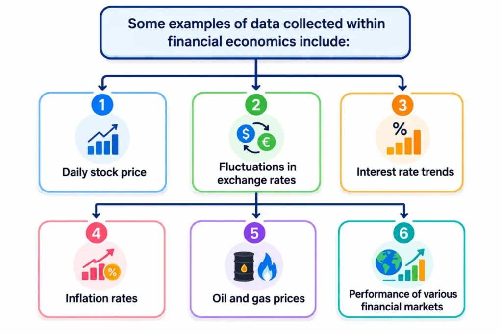
Some examples of data collected within financial economics include:
- Daily stock price
- Fluctuations in exchange rates
- Interest rate trends
- Inflation rates
- Oil and gas prices
- Performance of various financial markets
The purpose of looking at time series data is not just to understand what happened, but rather to utilize historical data to anticipate future changes. Utilizing historical data will empower financial professionals to make more informed decisions that rely on information as opposed to a guess or a hunch.
The Importance of Time Series Analysis in Financial Economics:
When making financial decisions, one must always deal with some level of uncertainty. Investors want to know the likely future movements in markets; businesses must assess their financial risks; and policymakers need to determine the general state of the economy before making new decisions.
Time series analysis gives a systematic way of putting order into these problems. By identifying trends and patterns in past data, businesses will have a better understanding of the dynamics of the market, leading to improved forecasts.
Time series analysis can help financial institutions and individual investors achieve the following advantages:
1) Better forecasts of financial variables
2) Easier to manage risks
3) Improved decisions regarding investments
4) Greater ability to understand market trends
5) More effective business planning.
The above advantages make it a useful tool in any financial economic institute or for individual investors [3].
The Use of Time Series Analysis in Financial Economics
1. Forecasting Stock Market Activity
Time series analysis enables investors to anticipate price movement and assess the possibility of investing
The following are the most advantageous uses of this application in terms of the results produced:
- Trend identification
- Price predicting
- Volatility evaluating
Investment planning improvement
2. Risk Management
By using past market data, financial institutions can analyze potential risks and to prepare for changes in the market.
The use of time series analysis benefits financial institutions by improving their ability to:
- Measure volatility in the market
- Assess potential losses
- Analyze risks associated with finance [4]
- Develop improved risk management strategies
3. Interest Rate Forecasting
Because of the effect interest rates have on lending, investing, and overall economic growth, time series models have been developed to assist with predicting interest rate trends.
Time series models enable analysts to do the following:
- Predict future interest rate trends
- Establish basis for effective financial planning
- Analyze impacts of monetary policy on interest rates
- Enhance decision-making processes by assisting with investment decisions
4. Predicting Exchange Rates
Businesses involved with international trade depend on forecasted exchange rates.
The benefits of using time series analysis for an organization involved with international trade include:
- Reducing the risk associated with currency exchanges
- Providing a basis for global investment
- Providing a basis for effective financial planning
- Reducing the uncertainty associated with international trade transactions
5. Portfolio Management
Portfolio managers utilize time series analysis to monitor their assets and make the most advantageous investments [3].
Benefits of employing time series analysis by portfolio managers are as follows:
- Allocating assets
- Diversifying portfolio investments
- Keeping track of portfolio performance
- Making predictions regarding portfolio returns
6. Economic Forecasting
Both organizations and businesses employ time series analysis for the purpose of making predictions regarding major economic indicators including inflation and gross domestic product growth.
Examples of the different ways in which various organizations employ time series analysis include:
- Economic development
- Implementing policy
- Assessing the market
- Economic forecasting.
There are many different analytical models being used to analyze certain types of financial problems [2].
| Model | Purpose | Common Use |
| ARIMA | (Autoregressive Integrated Moving Average) Forecast future value using previous trends of the asset | Stock price forecast |
| GARCH | (Generalized Autoregressive Conditional Heteroskedasticity) Analysis of volatility for the market | Risk management |
| Exponential Smoothing | Emphasizes only the most recent observations | Short-term forecasts |
| VAR | (Vector Autoregression) Analysis of the relationships between several different variables | Economic forecasts |
Analysts utilize these models to produce reliable predictions and have a better understanding of financial behavior.
The Evolution of Time Series Analysis in Finance
With the advancement of artificial intelligence, machine learning and large amounts of data, forecasting financial markets is becoming increasingly sophisticated.
Today, many organizations are integrating traditional time series models with AI-based approaches to:
- Enhance predictive ability
- Be able to work with greater volumes of financial information
- Identify latent patterns in the market
- Enable decision-making in real time
Time series analysis will continue to be a key area of research and support for financial markets as the technology advances.
Conclusion:
As one of the cornerstones of financial economics, time series analysis has assisted businesses, investors and researchers in gaining valuable knowledge of past behavior so that they can predict future behavior with greater accuracy.
Examples of the various applications of time series analysis are forecasting stock prices, hedging products, forecasting exchange rates and developing economic plans for a variety of financial industries [4].
The ability of organizations to use time series analysis in the rapidly evolving financial markets will enable them to access greater levels of information and ultimately improve their financial performance through more accurate decision-making.
At Statswork, we provide professional Data Analysis Services tailored to the unique needs of researchers, students, businesses, and financial professionals. Our team of statistical experts assists with data analysis, forecasting models, trend identification, and interpretation of results, ensuring accurate and reliable insights for your projects.
References
- Praveen, M., Dekka, S., Sai, D. M., Chennamsetty, D. P., & Chinta, D. P. (2026). Financial time series forecasting: A comprehensive review of signal processing and optimization-driven intelligent models. Computational Economics, 67(2), 963-989. https://link.springer.com/article/10.1007/s10614-025-10899-z
- Alsharef, A., Aggarwal, K., Sonia, Kumar, M., & Mishra, A. (2022). Review of ML and AutoML solutions to forecast time-series data. Archives of computational methods in engineering, 29(7), 5297-5311. https://link.springer.com/article/10.1007/s11831-022-09765-0
- Zamanzadeh Darban, Z., Webb, G. I., Pan, S., Aggarwal, C., & Salehi, M. (2024). Deep learning for time series anomaly detection: A survey. ACM Computing Surveys, 57(1), 1-42. https://dl.acm.org/doi/full/10.1145/3691338
- Fatima, S. S. W., & Rahimi, A. (2024). A review of time-series forecasting algorithms for industrial manufacturing systems. Machines, 12(6), 380. https://www.mdpi.com/2075-1702/12/6/380