Explain And Execute Statistical Design And Analysis Of Two Variable Hypothesis

In this blog, I will explain you how the statistical analysis is being applied for two independent samples. In practice, the test statistic used for comparing the two means from a population is by using the t-test because t-test shrinks the data to a single t-value and it is then compared with the significant value for the final conclusion. Now, Let us understand the theoretical background in performing the t-test for two variables.

Suppose X₁ and X₂ be the two independent random variable and let , be the sample with size n₁ and n₂ from a population with mean µ₁, µ₂ and variance σ₁², σ₂² respectively. It is obvious that if the sample size is large enough then the sample mean will follow a normal distribution, (i.e)

x ̅_1~N(μ_1,(σ_1^2)/n_1 ) and x ̅_2~N(μ_2,(σ_2^2)/n_2 )

In addition, if the means of the two samples are said to follow normal distribution, then the difference of mean are also said to follow normal distribution. It is given by

Z=((x ̅_1-x ̅_2 )- E(x ̅_1-x ̅_2))/(S.E.(x ̅_1-x ̅_2 ) )~N(0,1)

Under the null hypothesis, H₀: µ₁ = µ₂ which means there is no statistical significant difference between the means. The test statistic becomes

Z=((x ̅_1-x ̅_2 ))/√((s_1^2)/n_1 +(s_2^2)/n_2 )~N(0,1)

If suppose we come across the data having the same variance then the test statistics boils down to

Z=((x ̅_1-x ̅_2 ))/(s*√(1/n_1 +1/n_2 ))~N(0,1)

Once the t-value is calculated, the next step is to compare with the critical value with alpha level of significance and if the calculated t-value is less than the significant value then the conclusion is to reject the null hypothesis stating that there is a significant difference between the means of the population. (Cressie & Whitford, 1986)

Imagine a marketing company has recently launched two campaigns for advertising their product. The company’s head wants to identify whether both the campaign is equally effective or not. In such case, the statistical hypothesis testing is the essential method to give a valid inference. Before performing any statistical hypothesis testing, the main task is to understand the problem statement, to frame the hypotheses of interest, to find a suitable test statistics, and finally to make a proper decision with the results.

This blog will elaborate each one with the advertising example as mentioned above.

Understanding the Problem Statement

The primary or basic task in any statistical data analysis is to know or find out what the problem is and how the data is being measured. In our example, the manager wish to find the effectiveness of their campaign, for this, he/she has to consider all the information related to the campaign and find out whether the campaign results in a profit or loss. The only way to test whether the two campaign is effective is to perform a statistical test by comparing their means. 

Construction of Test Hypotheses

Once you understand the problem at hand, the next step is to frame an appropriate hypothesis to test for statistical significance; we call it as the null hypothesis and alternative hypothesis (Flandin & Friston, 2019). The null hypothesis is something which we claim or our belief about the problem and is denoted by H₀. That is, for our example, the null hypothesis will be there is no statistically significant difference between the mean incomes from two campaigns.

H₀:μ₁ = μ₂

Or

H₀:μ₁−μ₂=0

The alternative hypothesis (H₁) is simply a contrary to the null hypothesis. That is, there is a significant difference between the means of the two campaigns.

H₁: μ₁≠μ₂

or

H₁: μ₁−μ₂≠0

Finding a Suitable Test Statistics

For finding the suitable statistic test, we need to find the distribution of the data. I will illustrate with a simulated data for two campaigns using R software.

set.seed(123)

camp1<-rt(30,29)*50+210 camp2<-rt(30,29)*48+170           

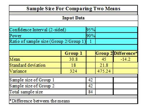
If you see the above graph, the data is closely from a normal distribution. However, I have taken the sample size as 30 per campaign, so we should make use of the t-distribution for testing this problem. From the simulated data, the mean for two campaigns is $210.2226 with standard deviation $60.0008 and $182.8537 with standard deviation $47.56557 respectively.

Calculation of test statistic

Once you got all the necessary values for the calculation, the next step is to apply it into the formula of statistics test as mentioned earlier. Here, I will illustrate using R.

Difference<-mean(camp1)-mean(camp2)

Std.dev<-sqrt((sd(camp1)^2+sd(camp2)^2)/2)

Std.err<-Std.dev*(1/length(camp1)+1/length(camp2))^0.5

t.value<-Difference/Std.err

The difference of mean is $27.3689 and the t-value is 1.9578.

Conclusion of the Problem

As a final step, we compare the calculated t.value with the critical value. In order to find the critical value, we need to fix the significance level alpha. Usually, it is considered as 5% that means we can tolerate the probability of rejecting the null hypothesis by 5% or 0.05 level of significance. Next step is to check whether the null hypothesis is one-sided or two-sided for the concluding the problem. If you are concerned about which campaign is higher or smaller then the null will be one-sided. However, in our case, it is two sided null hypothesis stating that the means of the campaigns are equal. An important note is that in a two-sided test the critical region is divided by half (5% is equally distributed in both sides from population mean).

The rejection region can be calculated using the confidence interval. If the t-value lies outside the confidence limit we will reject the null hypothesis otherwise we accept the same. In R, there is a function called t.test to perform the calculation and the p-value is compared with 0.05 for the conclusion.

Res<-t.test(camp1,camp2,paired=FALSE,var.equal=TRUE)

Res

        Two Sample t-test

data:  cam1 and cam2

t = 1.9578, df = 58, p-value = 0.05507

alternative hypothesis: true difference in means is not equal to 0

95 percent confidence interval:

 -0.613592 55.351410

sample estimates:

mean of x mean of y

 210.2226  182.8537

From the results, the t-value (or test statistic) is 1.9578 as we got previously and the p-value is 0.05507, which is greater than 0.05. Since the p-value is greater than 0.05, we accept the null hypothesis and conclude that the difference of mean amount from two campaign is same.To sum up, this blog is to elaborate and explain you the procedure used to test the two variables and how to provide a valid inference from the results. I hope this blog serves you better for understanding and analyzing similar data.

References

- Cressie, N. A. C., & Whitford, H. J. (1986). How to use the two sample t‐test. Biometrical Journal, 28(2), 131–148. Retrieved from https://onlinelibrary.wiley.com/doi/abs/10.1002/bimj.4710280202
- Flandin, G., & Friston, K. J. (2019). Analysis of family‐wise error rates in statistical parametric mapping using random field theory. Human Brain Mapping, 40(7), 2052–2054. Retrieved from https://onlinelibrary.wiley.com/doi/abs/10.1002/hbm.23839