Ordinary-least-squares (OLS) regressions are employed to determine whether relations exist between leverage ratio and determinants. Eviews 6.0 software developed by Quantitative Micro Software is used to analyze the OLS regressions. Two regression equations is used to test the hypotheses which are looking at firm specific determinants (PROFIT, GROWTH, NDTS and SIZE) and later add the country-specific determinants (BANK, STK, GDP and INF) to the first equation. The model of regression equation is as follows:

Where α = constant, β1 to Β8 = coefficient of explanatory variables, PROFIT = Profitability; GROWTH = Growth opportunities; NDTS =non-debt tax shield; SIZE = firm size; BANK = size of banking industry; SKTMKT = size of stock market; GDPRATE = GDP growth rate; and INF = annual inflation rate. ε is the error term
The first regression equation is to determine the firm-specific factors influencing leverage in the individual countries whereas the second regression is to examine the country effect on the leverage. This approach is consistent with previous studies as in Deesomsak et al. (2004) and Song & Philippatos (2004).
Rationale of the statistical analysis
Stationarity tests
The regression model as stated above should be estimated after conducting the Stationarity test which analyse the most appropriate form of the trend in the data. Prior to analysis, particularly when using ARMA modelling the data must be transformed to stationary and trend needs to be removed. The test was conducted in order to identify the presence of unit roots (trending data) in all variables included in the study. In the present study researcher adopted “Augmented Dickey-Fuller (ADF) test” by Dickey and Fuller (1979). This test is used to check for the homoscedasticity of residual errors and independency (or deterministic, stochastic or combination of both).
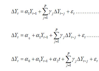
The Augmented Dickey Fuller (ADF) test (1979, 1981) is used for this purpose. The three different ADF Regression equations are

Where et is white noise. The additional lagged terms are included to ensure that the errors are uncorrelated. The tests are based on the null hypothesis (H0): Yt is not I (0). If the calculated DF and ADF statistics are less than their critical values from Fullers table, then the null hypothesis (H0) is accepted and the series are non-stationary or not integrated of order zero.
In the second step we estimate co integration regression using variable having the same order of integration. The cointegration equation estimated by the OLS method is given as Yt = a0 + a1 Xt + zt
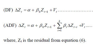
In the third step residuals (Zt) from the cointegration regression are subject to the Stationarity test based on the following equation.

The sequential procedure involves testing the most general model first. Since the power of the test is low, if we reject the null hypothesis, we stop at this stage and conclude that there is no unit root. If we do not reject the null hypothesis, we proceed to determine if the trend term is significant under the null of a unit root. If the trend is significant, we retest for the presence of a unit root using the standardized normal significant, we retest for the presence of a unit root using the standardized normal distribution. Otherwise it does not. If the trend is not significant, we estimate equation and test for the presence of a unit root. If the null hypothesis of a unit root is rejected, we conclude that there is no unit root and stop at this point. If the null is not rejected, we test for the significance of the drift terms in the presence of a unit root. If the drift term is significant, we test for a unit root using the standardized normal distribution. If the drift is not significant, we estimate equation (10) and test for a unit root.
Data Analysis Plan for TARCH (Threshold ARCH):
Traditionally, financial variables always tend to change over time and always smaller changes tend to follow the large changes and vice versa. In the dependent variables, episodes of volatility are generally characterized by large shocks. In order to mimic this phenomenon the conditional variance function is formulated. In the model of regression, from its conditional mean or equivalently a large positive or negative value of error term, a large deviation of dependent variable is represented through a large shock. An irrespective of the signs, the variance of the current error in the ARCH regression model shows an enhanced function of the lagged errors magnitude. Thus, a large error to either sign is followed through the smaller errors of either sign. And similarly, a small error to either sign is followed through the large error of either sign. In conditioning the variance of subsequent errors, the order of the lag q determines the length of time for which a shock persists. Further, if the value of Q tends to be larger, then the volatility will also tend to be larger.
The researcher has to exercise caution when distinguishing between good news and bad news in the financial markets. Bad news depresses asset prices and historically leads to these Foreign Portfolio Investors to exit the financial markets and conversely, good news leads to asset price appreciation attracting portfolio investors (Agarwal,R.N. 1997). (Kulwant Rai, N.R Bhanumurthy 2004) and (Kumar Sundaram 2009) (Chakrabarti Rajesh) have proved that the sensitivity with which these investors withdraw is greater than the sensitivity with which they invest. On account of being more risk averse in nature, their speed in investing is relatively slower than their speed in pulling out their investments from the markets. This leads to asymmetry between good and bad news. (Kulwant Rai, 2004)
At the 5% significance levels the null hypothesis could be rejected and similarly if the p value was greater than α = 5% which at the 5% significance levels, the alternative hypothesis was rejected.
 Celebrate the season with exclusive savings from Statswork!


