SEM using AMOS Statistical Services from Experts at Stats work

Structural Equation Modeling (SEM) is an extension of the general linear model. It is used to test a set of regression equations simultaneously. The advantages of SEM Analysis are as follows:

• SEM provides overall tests of model fit and individual parameter estimate tests simultaneously.
• Regression coefficients, means and variances may be compared simultaneously.
• It is the graphical interface software.

SEM represents the relationship between dependent (unobserved) variable and independent (observed) variables using path diagrams. In this analysis, ovals or circles represent dependent variable and rectangles or squares represent independent variable. Residuals (error term) variables also represent by ovals or circles, because they are always unobserved. Statswork experts are well-versed in conducting SEM analysis for your research works. We have a team of expertise who are experienced in handling a number of SEM analysis for the past ten years.

What Statistical consultation Services we offer at SEM analysis?

With the holistic approach, the statistical consultation services at Statswork provides an overall view about your research work and we ensure to provide you the output of the SEM model that correlates with your research framework. Here is how we proceed and provide you the final output for the SEM analysis.

What are the values are extracting from this test?

If the hypothesized model has a good fit, the statistical test values should be in the following manner.

• Chi-square value should be less than 5
• P value should be greater than 0.05
• GFI, AGFI and CFI values should be greater than 0.90
• RMR & RMSEA values should be less than 0.08

The output and their description are as follows:

First order CFA model only contains the residuals, items (questions) with corresponding factors (independent). But in the second order CFA model has the overall model fit for dependent variable and independent variable.

First- order CFA model

In contrast to a first-order CFA model, which comprises only a measurement component, and a second –order CFA model for which the higher order level is represented by a reduced form of structural model, hence the full structural equation model comprises of both a measurement and structural model. In the full SEM model, certain latent variables are connected by one way arrows, the directionality of which reflects hypotheses in the study bearing on causal structure of variables in the model.

Full data (Both Organized and Unorganized retailer)

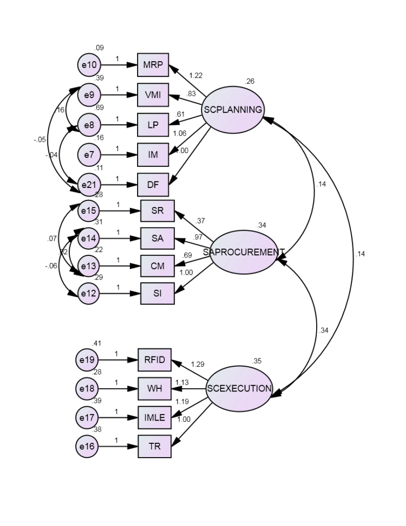
In the first order model, the modification Indices is higher in Reverse Logistics so that factor is removed from the model.

Figure 1: First-order model for Supply Chain Planning, Sourcing and Procurement and Supply Chain Execution

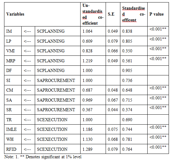
Table 1: CFA for First-order Model for dimensions of Supply Chain Planning, Sourcing and Procurement and Supply Chain Execution

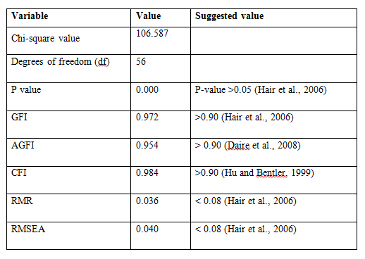
To examine the theoretical interdependence between three factors (Supply Chain Planning, Sourcing and Procurement, Supply Chain Execution) structural equation modelling was used. This analysis allows to test all the relevant paths and measurements errors and feedbacks are included directly into the model. The fit indices show an adequate fit as the factors are found to be significant at the p<0.05 (Table 2). The model fit, which was assessed using global fit (seven different fit indices) and ‘r’ to identify the degree to which the hypothesized model is consistent with the data in hand. In other words, the degree to which the implicit matrix of co variances, (based on the hypothesized model), and the sample covariance matrix, based on data it seems to fit (Bollen, 1989).The structural model, the quality of fit was acceptable representation of the sample data (χ2 (560)= 106.587, GFI (Goodness of Fit Index)=0.972; AGFI (Adjusted Goodness of Fit Index) = 0.954 which is much larger than the 0.90 criteria as suggested by Hu and Bentler (1999) and Joreskog and Sorbom (1981). Similarly, CFI=0.984, RMSEA (Root Mean Square Error of Approximation) =0.040 and RMR (Root Mean Square Residuals) =0.036, values are lower the 0.05 critical value (Steiger, 1989).

Table 2: Model fit summary

Second-order model (Operational Performance as dependent variable)

Full data (Both Organized and Unorganized retailer)

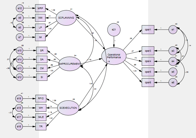
In the second order model, if the modification Indices is higher then error terms are related and also in the independent variables Demanding forecasting, Reverse Logistics factor is removed from the model and in dependent variable Operational performance (Item no. 2) is removed due to low correlation.

Figure 2: Second-order model for Supply Chain Planning, Sourcing and Procurement and Supply Chain Execution with Operational Performance

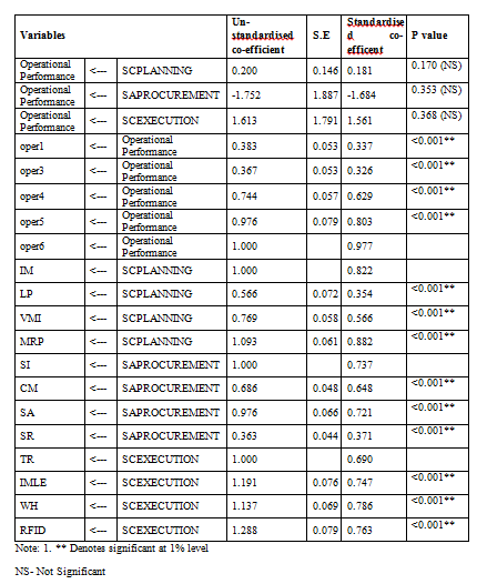
Table 3: Second-order Model for dimensions of Supply Chain Planning, Sourcing and Procurement and Supply Chain Execution with Operational Performance

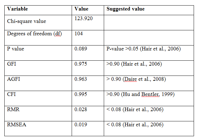
To examine the theoretical interdependence between three factors (Supply Chain Planning, Sourcing and Procurement, Supply Chain Execution) with Operational Performance as a dependent variable, structural equation modelling was used. This analysis allows to test all the relevant paths and measurements errors and feedbacks are included directly into the model. The fit indices show a model is good fit as the factors are found to be significant at the p>0.05 (Table 4). The model fit, which was assessed using global fit (seven different fit indices) and ‘r’ to identify the degree to which the hypothesized model is consistent with the data in hand. In other words, the degree to which the implicit matrix of co variances, (based on the hypothesized model), and the sample covariance matrix, based on data it seems to fit (Bollen, 1989).The structural model, the quality of fit was acceptable representation of the sample data (χ2 (560)= 123.920, GFI (Goodness of Fit Index)=0.975; AGFI (Adjusted Goodness of Fit Index) = 0.963 which is much larger than the 0.90 criteria as suggested by Hu and Bentler (1999) and Joreskog and Sorbom (1981). Similarly, CFI=0.995, RMSEA (Root Mean Square Error of Approximation) =0.019 and RMR (Root Mean Square Residuals) =0.028, values are lower the 0.05 critical value (Steiger, 1989).

Table 4: Model fit summary

What you will get when you order for SEM statistical consultation services at Stats work: Our Service description

On which areas you provide SEM analysis

We accept orders from a wide range of subjects which include Business Management, Economics, Epidemiology, Public Health, Life Science, and Nutrition

What Information that I need to provide while ordering for SEM statistical analysis consultation services

The data must contain without any missing value. To match exactly with your requirement, we required title that you had already selected objectives and research questions.