Application of Logistic Regression using R Programming
Application of Logistic Regression using R Programming
Experience of Statswork.com
In this blog, we will look into the practical application of Logistic Regression using R in detail. Performing Logistic Regression is not an easy task as it demands to satisfy certain assumptions as like Linear Regression. Before reading further, I would suggest you read and understand how Linear Regression works.
Now, let us understand what Logistic regression is.
Logistic Regression Analyses
Suppose you have a medical data to predict the medical condition of a patient having high blood pressure (BP) or not along with other observations such as Age, Smoking habits, Weight, or Body mass Index BMI, blood cholesterol levels, Diastolic and Systolic BP value, Gender, etc.
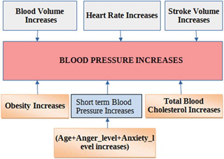
Source: adapted from Nimmala et al., 2018
First thing you do is to select the response or dependent variable, and in this case, patients having high BP or not will be response variable or dependent variable (refer Table 1 for cut-off) and others are explanatory or independent variables. Dependent variable needs to be coded as 0 and 1 while explanatory variable can be a continuous variable or ordinal variable.
| Table 1. Blood pressure range | ||||
| BP | Low | Normal | Borderline | High |
| Systolic | <90 | 90–130 | 131–140 | 140 |
| Diastolic | <60 | 60–80 | 81–90 | >90 |
In such a scenario, one wishes to predict the outcome by applying suitable model namely the logistic regression model.

Definition:
Logistic regression is a type of predictive model which can be used when the target variable is a categorical variable with two categories. Logistic regression is used for the prediction of the probability of occurrence of an event by fitting the data into a logistic curve. Like many forms of regression analysis it makes use of predictor variables, variables may be either numerical or categorical.
Logistic regression is to predict the presence or absence of a characteristic or outcome based on values of a set of predictor variables while in this case prediction of high BP. It is suitable for models where the dependent variable is dichotomous. Logistic regression coefficients can be used to estimate odds ratios (OD) for each of the independent variables in the model.
The main aim of logistic regression is to find the best fitting model to describe the relationship between the dichotomous characteristic of interest and a set of independent (predictor or explanatory) variables. Simply, it predicts the probability of occurrence of an event by fitting data to a logit function.
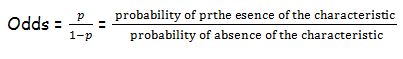
Logistic regression generates the coefficients of a formula to predict a logit transformation of the probability of the presence of the characteristic of interest:
Logit (p) = b0 + b1X1 + b2X2 +…+ bkXk
where p is the probability of the presence of the characteristic of interest. The logit transformation is defined as the logged odds:

Rather than choosing parameters that minimize the sum of squares. The table below shows the prediction model for childhood high blood pressure
Table 1. Prediction model for childhood high blood pressure.
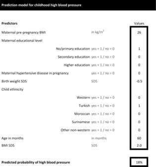
Adapted from Hamoen et al., 2018
Logistic regression in R
R is an easier platform to fit a logistic regression model using the function glm(). Now, I will explain, how to fit the binary logistic model for the Titanic dataset that is available in Kaggle. The first thing is to frame the objective of the study. In this case, one wishes to predict the survival variable with 1 as survived and 0 as not survived along with other independent variables.
Primary step is to load the training data into the console using the function read.csv ().
train.data<- read.csv(‘train.csv’,header=T,na.strings=c(“”))
Before going to the fitting part, one should check whether there exists missing data. It can be achieved by sapply() function in R.
sapply(train.data,function(x) sum(is.na(x)))
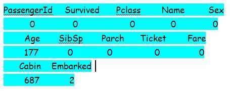
From the above result of the sapply function, we can see that the variable “cabin” has many missing entries. ,Also, the variable “PassengerId” contains missing data. We will skip these two variables for the analysis as it is not relevant to the objective of the study.
We can omit those variables and make a subset of the data as new with the subset () function.
data <- subset(train.data,select=c(2,3,5,6,7,8,10,12)) where the numeric values in the select argument is the columns in the data file.
Next step is to check for other missing entries in the subset data. There are different ways to replace the NA’s with either the mean or median of the data. Here, I used the mean for replacing NA’s like
data$Age[is.na(data$Age)] <- mean(data$Age,na.rm=T)
Fitting Logistic Regression Model
Before fitting the model, we split the data into two sets, namely training and testing set. The training set is used to fit the model where the latter is used for testing purpose.
traindata<- data[1:800,]
testdata<- data[801:889,]
Let’s start fitting the model in R and make sure you specify family = binomial in glm() function since our response is binary.
lrmodel<- glm(Survived ~.,family=binomial(link='logit'),data=traindata)
The result of the model can be obtained using the following command:
summary(lrmodel)
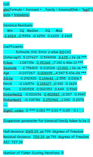
The next serious part is to interpret the result of the model. From the p-value of the summary of the model, the variable Embarked, Fare, and SibSp are not statistically significant. Also, the variable sex has lesser p-value, which means there is a strong association of passengers with the chance of survival.
It
is important to note that the response variable is log odds and can be written
as ln(odds) = ln(p/(1-p)) = a*x1 + b*x2 + … + z*xn.
To analyse the deviance, we should use ANOVA() function in R.
anova(lrmodel, test=”Chisq”)
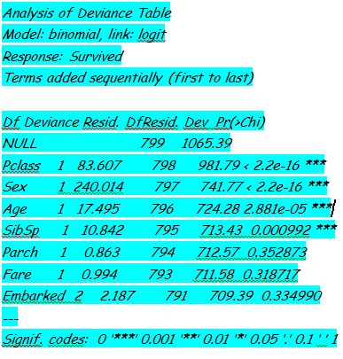
The difference between the null deviance and the residual deviance explains the performance of the model against the null model (a model with only the intercept). If the difference is wider, model performs better. Large p-value indicates that the logistic regression model without that particular variable explains the same amount of variation. At the end, one can infer that lesser AIC is the best model.
Next important step is to predict the model on a new set of data and R enables us to do with predict() function. Let us consider our threshold for the new response data. That is, if P(y=1|X) > 0.5 then y = 1 otherwise y=0. The threshold could be changed according to the researchers needs. The following Table presents the accuracy prediction formulas especially when machine learning algorithms are applied.
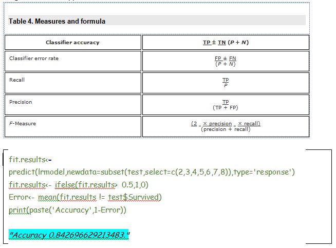
84.26% of accuracy is actually a good result. Note here; I have split the data manually, if you split the data in a different way, then the accuracy of the model will alter.
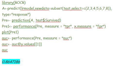
Finally, we find the area under the curve by plotting ROC curve using the following commands. ROC curve generates the true positive rate against false positive rate, similar to the sensitivity and specificity. If the AUC is closer to 1, then we get a good predicting model.

Well. we come to the end of this tour! I hope now you can analyse logistic regression using R on your own. Further, I suggest you try the same Titanic datasets and check you get the same results before exploring other datasets.
References
- Richard A. Johnson and Dean W. Wichern (1992), Applied Multivariate Statistical Analysis. Pearson Prentice Hall.
- W. Hosmer, Jr., Stanley Lemeshow (2004). Applied Logistic Regression, 2nd Edition, John Wiley and Sons.
- R Core Team (2013). R: A language and environment for statistical computing. R Foundation for Statistical Computing, Vienna, Austria.
- Joseph M. Hilbe (2015). Practical Guide to Logistic Regression. CRC Press.
[wce_code id=1]
 Previous Post
 Next Post