

Quantile Regression in STATA. Few Advantages of the Model with Example.
The traditional linear regression provides the relationship between the regressors and the response variable based on the conditional mean. This type of regression explain the relationship partially because the researcher may not describe the relationship at different points of y. This drawback is nullified by the quantile regression and it uses the conditional median function instead of mean function. As we all know, median is the 50% of the data or a quantile q = 0.5 or the 50th percentile of the data i.e F(yq) = q then yq = F-1(q).
The main task of any regression analysis is to minimize the error term. Unlike in usual regression method, the quantile regression or the median regression or the least absolute deviations (LAD) minimizes the sum of absolute value of the prediction error, i.e .
One of the main advantage of using quantile regression is that it will take care of the over-dispersion and under-dispersion in the data. That is, it minimizes the error with (1-q)*|ei| for over dispersed data and q*|ei| for the under dispersed data. The other advantages of using median regression is that
- it is more robust or less sensitive to outliers than OLS estimates
- No assumptions about the distribution of the parameters.
- If the errors are non-normal then OLS may be inefficient. But QR is more robust to non – normal data and outliers.
- It allows to consider the impact of covariates of y
- It is invariant to monotonic transformations
- It is also suitable for count data types using Poisson regression.
- Resistant to outliers.
Like in usual regression model, the quantile regression model can be expressed as
Where yi is the outcome variable, xi is the explanatory variables, βq is estimated value and Єi is the error term. Then the quantile regression estimator minimizes the following objective function.
The quantile regression uses the linear programming method in contrast to the maximum likelihood as in usual linear regression method.
Let me illustrate the quantile regression using a medical expenditure data analysis using STATA. Here, the response variable is the total medical expenditure of the people surveyed and the independent variable are the age, gender specifically female, white, insurance, and the health status. There are few missing entries present in the data and are omitted for the analysis.
The following table gives the descriptive summary of the variables under study.
| Variable | Obs | Mean | Std. Dev. | Min | Max |
| ltotexp | 2955 | 8.0598 | 1.3675 | 1.098 | 11.7409 |
| ins | 2955 | 0.5915 | 0.4916 | 0 | 1 |
| totchr | 2955 | 1.8087 | 1.2946 | 0 | 7 |
| Age | 2955 | 74.2453 | 6.3759 | 65 | 90 |
| Female | 2955 | 0.5840 | 0.4929 | 0 | 1 |
| White | 2955 | 0.9736 | 0.1603 | 0 | 1 |
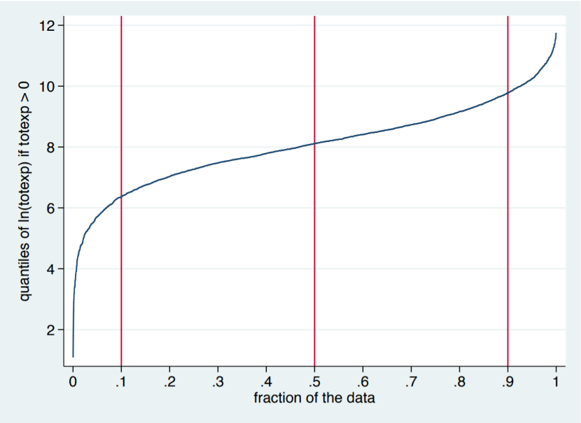
Next, we plot the CDF of the log of the response variable to check whether it is symmetric in nature.
. qplot ltotexp, recast(line) ylab(,angle(0)) /// xlab(0(0.1)1) xline(0.5) xline(0.1) xline(0.9)
The next step is to conduct the median regression with all covariates. In STATA, this can be done using the qreg function.
. qreg ltotexp ins totchr age female white, nolog
The result as follows:
Raw sum of deviations = 3110.961 (about 8.111928) Number of obs = 2955
Min sum of deviations 2796.983 Pseudo R2 = 0.1009
| ltotexp | Coef. | Std. Err. | t | P>|t| | [95% Conf. Interval] |
| ins | 0.277 | 0.0536 | 5.17 | 0.000 | .1718924 .3820617 |
| totchr | 0.3943 | 0.0202 | 19.47 | 0.000 | .3545663 .4339664 |
| age | 0.0149 | 0.0041 | 3.58 | 0.000 | .0067335 .0229996 |
| female | -0.088 | 0.0532 | -1.66 | 0.098 | -.1924109 .0162175 |
| white | 0.4987 | 0.1631 | 3.06 | 0.002 | .1789474 .818544 |
| _cons | 5.6489 | 0.3412 | 16.56 | 0.000 | 4.979943 6.317838 |
From the p-value, it is clear that only the covariate female is statistically significant from the QR model.
Next, we will calculate the marginal effects on the response variable for this study.
| ins | totchr | age | female | white | _cons | |
| y1 | 1037.755 | 1477.2049 | 55.701 | -330.0735 | 1868.65 | 21164.8 |
From this marginal effects, we infer that there is an increase in expenditure by $1477.20 if the expenditure increased by $55.70 per year.
In order to find the efficiency of the QR regression, we now compare it with the usual OLS regression at various quantiles.
- . eststo clear
- . eststo, ti(“OLS”): qui reg ltotexp ins totchr age female white, robust
- (est1 stored)
- . foreach q in 0.10 0.25 0.50 0.75 0.90 { 2. eststo, ti(“Q(`q´)”): qui qreg ltotexp ins totchr age female white, q(`q´) nolog 3. }
- (est2 stored)
- (est3 stored)
- (est4 stored)
- (est5 stored)
- (est6 stored)
The result of the comparative study is tabulated below.
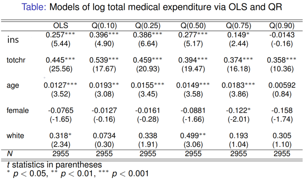
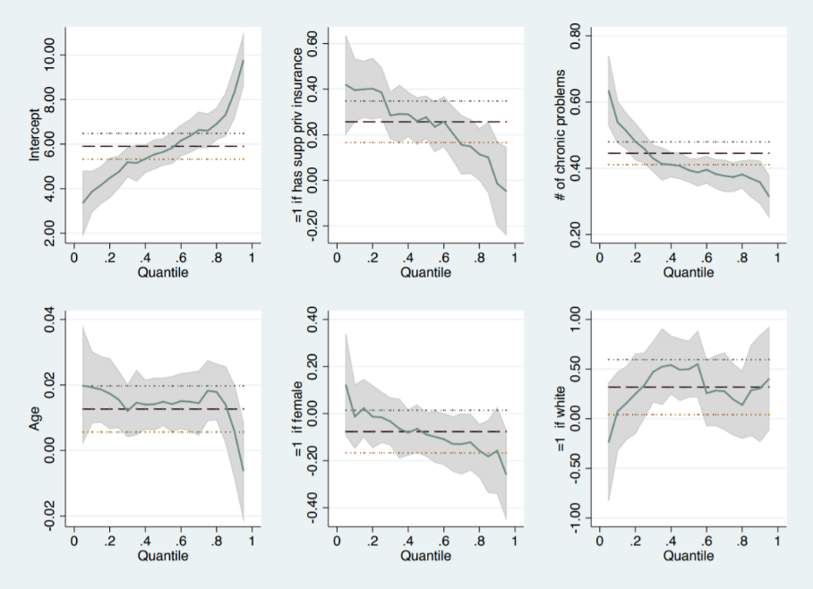
From the above result, it is clear that the insurance have a big effect on total expenditure when the quantiles are less. The median quantile results similar to the OLS. In the same way, we can also identify how each covariates differs in each quantile using STATA. The following graph shows how the covariates differs in each quantile.
In conclusion, Quantile regression provides an alternative to OLS regression based on the conditional median, that is, it identifies the relationship between the variables beyond the mean data points. It is more appropriate when the data are not normally distributed and if it contains the observations that are more influential and it is more robust to outliers.
- Buchinsky M. Recent advances in quantile regression models: a practical guideline for empirical research. Journal of Human Resources. 1998;33(1):88–126.
- Koenker R. Quantile Regression. Cambridge, UK: Cambridge University Press; 2005.
- https://sites.google.com/site/econometricsacademy/econometrics-models/quantile-regression
 Previous Post